In this article
- What you will learn
- Where the question came from
- How we measured it
- The result
- Step 1 · 48%: a threshold the size of an ordinary week
- Step 2 · 8%: quiet for the wrong reason
- Step 3 · 11%: every day against its own kind
- The formulas, on a worked example
- The most common mistakes
- The lesson: the number went down, then back up
- Beyond football: alarm fatigue
- What sport science says
- What we don't know
What you will learn
- Why a fixed percentage threshold fires on ordinary days when it is smaller than the noise of the measure.
- How to work out a against an athlete's norm, and why the threshold has to rise when the norm rests on few days.
- How to judge an alert rule: not only how many alerts it raises, but where they fall.
Where the question came from
The scene is always the same. Monday meeting, the weekend's sheet on the table, half the squad coloured in. Nobody asks a question. Then someone turns the page: "It's always all red anyway."
Anyone who has built a monitoring panel knows the sequence: at first every colour gets discussed, after a few weeks there are too many colours, after a month the panel is wallpaper. It is not laziness: it is the rule that decides when a colour comes on.
This dossier is about one of those rules, and it is ours. In its first version MarkerDrift used the thresholds you find more or less everywhere, 10% and 20%. Measured over a whole season, it lit up almost one day in two. The obvious fix went wrong in a different way. The third version is today's.
How we measured it
The data. The simulated 2026/27 season of FC Demo, MarkerDrift's demo club: 25 invented players, no real athlete and no real club. One metric only, GPS total distance summed over the day: one row per athlete-day, 7,766 athlete-days, 6,898 without absences.
Kinds of day. Every day has a (MD is the match, MD-1 the day before, MD+1 the day after) and a kind: training, match, rest, absent, not measured. Absences are the demo's 9 injury periods plus any run of 7 or more days without a measurement. A rest day counts as 0 m; a training day without a measurement is a gap, not a zero, and like an absence it never enters a reference.
The three rules.
- A, before. The day's distance against the median of the last 3 days with the same MD label (a match only against matches). Amber from a 10% change, red above 20%, up or down. Rest days are judged like any other day.
- B, the first fix. A z-score against the athlete's previous 28 days, at least 8 values, with every kind of day in the norm, rest days at 0 m included. Amber from 1.5 standard deviations, red above 2.0. A rest day is not judged.
- C, today: the "work norm". Each training or match day against the same athlete's last 8 days with the same MD label and the same kind, looking back at most 120 days; until there are 8, the previous 28 days of the same kind. Thresholds from 1.5 and 2.0, corrected for the sample.
How we counted. Only days with a complete reference: for rule A, all three matching days found; for B and C, no absence inside the window. Counting every day a rule can judge moves the figures only slightly: 49.6%, 8.6% and 11.0%.
The check. An independent script gives the same verdicts as the app's own engine, day by day: zero differences out of 39,738. The data and the calculation can be downloaded here, no sign-up needed: dossier-48-dati.zip (the CSV, the script and the instructions).
The result
| A · before | B · first fix | C · today | |
|---|---|---|---|
| Days judged | 5,257 | 4,080 | 4,765 |
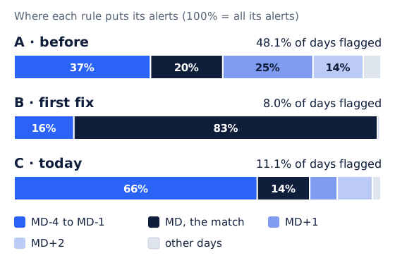
| Days flagged | 48.1% | 8.0% | 11.1% |
| Reds per amber | 1.06 | 0.79 | 0.45 |
| Alerts per athlete per week | 2.56 | 0.33 | 0.54 |
| Share of alerts on match days | 19.7% | 82.8% | 14.3% |
| Matches flagged (808 measured) | not counted | 43.4% | 9.4% |
| Alerts in the 21 days after 8 returns | not counted | 9 | 35 |
For rule A, matches and returns are not counted on the same basis: of the matches it judges, it flags 67.8%.
Step 1 · 48%: a threshold the size of an ordinary week
Rule A flags 2,526 days out of 5,257. There are more reds than ambers (1.06 per amber), which is odd in itself: red is supposed to be rare. For one athlete that is 2.6 alerts a week; for the staff of a 25-man squad, dozens of colours every Monday.
Part of it is explained at once: all 465 rest days judged are red, because 0 m against three working days is −100%. They make up 18% of the alerts. But even without judging rest days the rule still flags 43.0% of days.
The rest is noise. Over the season a player's distance on the same training MD varies with a median of 11%: about 8% from MD-3 to MD-1, 19.5% on MD-4, 30% on MD+2 and 40% on MD+1, the day after the match, when the squad splits between those who played and those who did not. On days that are not rest days the median change from the reference is 8.5%, and only 57% stay within ±10%.
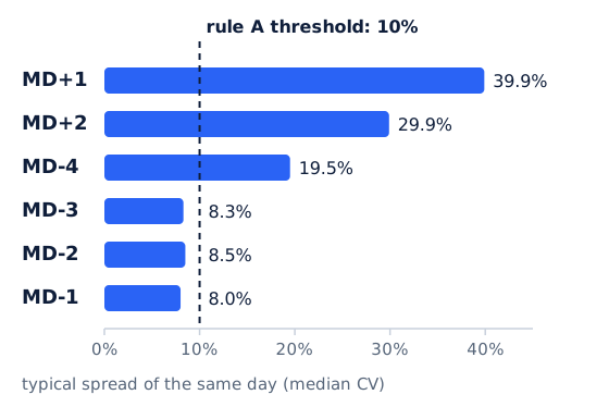
A 10% threshold, in other words, is roughly how much an ordinary day moves: on the steadiest days it fires one time in three (31.9% from MD-4 to MD-1), on the day after the match almost always (86.1%). Of the 1,538 non-rest days that rule A flags and rule B can also judge, 90% sit inside the athlete's own norm. The flaw is the idea that one number fits every day and every athlete.
Step 2 · 8%: quiet for the wrong reason
The obvious fix is to express the day's distance in standard deviations of the athlete's own norm. With rule B the alerts drop to 8.0% (326 out of 4,080), 0.33 per athlete per week. Just what we wanted to see.
Then we looked at where they fell: 82.8% on match days, with 43% of the 808 measured matches flagged. On training days almost nothing, 2% of the days judged.
The reason lies in the norm. Twenty-eight days hold training sessions, three or four matches and rest days at 0 m: the mean drops and the standard deviation swells. The match, the day with the most metres of the week, falls outside that norm almost by definition (telling us that a match is not a training session, which we knew), while a training day, even one very different from usual, stays inside such a wide band.
The returns gave it away. The simulated season has 8 returns after an injury absence. In the 21 days after each return rule B gave 9 alerts in all, out of 100 days judged, and three athletes had none. And all 9 were days above the norm: the reduced load of the first sessions back, exactly what a staff wants to see written down, never appeared. A low rate, here, meant a rule looking at the wrong thing.
Step 3 · 11%: every day against its own kind
Rule C asks a narrower question: is this day far from his usual for this kind of day? An MD-3 training session against his last eight MD-3 training sessions, a match against his last eight matches, never a rest day in a training norm. Eight matching days take about ten weeks to build up (over the season: 3,386 days judged that way, 1,670 against the window).
The second change is the thresholds. A mean and a standard deviation from 8 values are uncertain estimates, and a new value falls outside ±1.5 standard deviations more often than the normal curve says. The threshold is corrected with Student's t (the quantile with n − 1 degrees of freedom, times √(1 + 1/n)): with 8 values amber starts at 1.80 and red at 2.58; with 20 values at 1.61 and 2.19.
The result is 11.1% (531 out of 4,765), with 0.45 reds per amber. Match days carry 14.3% of the alerts, and flagged matches drop from 43% to 9%. Two thirds of the alerts (66.3%) fall from MD-4 to MD-1, the days on which the staff builds the week.
Now the returns show: in the same 21 days the alerts go from 9 to 35 (out of 113 days judged), at least two for every return, and 27 of the 35 are days below his usual: the reduced load of the first sessions back, read against the norm from before the absence. It is a description: it tells you the return was gradual, not how the athlete is. And in a quiet month it stays quiet: a demo player with no absence all season has one alert in 15 days judged in February (rule B gave him two, both on match days).
The price, stated up front. Compared with rule B the alerts rise from 8.0% to 11.1%, about three points. And the eight matching days have to be waited for: an athlete's first matches stay n/a until there are eight to compare them with, so 74% of match days are judged (87% under rule B); among measured working days, those without a verdict rise from 10.6% to 12.3%.
The formulas, on a worked example
An invented example, so you can follow the three calculations by hand. One athlete, total distance on an MD-3.
Rule A, the percentage change. The last three MD-3s were 5,200, 5,300 and 5,450 m: the median is 5,300 m. Today he covers 5,850 m.
change = (5,850 − 5,300) ÷ 5,300 = +10.4% → amber (above 10%)
Rule C, the z-score against the work norm. His last 8 MD-3s have a mean of 5,200 m and a standard deviation (sample, with n − 1) of 300 m.
z = (5,850 − 5,200) ÷ 300 = +2.17
With the written thresholds (1.5 and 2.0) that would be red. But the norm rests on only 8 days, and the thresholds corrected for the sample become 1.80 and 2.58:
1.80 ≤ 2.17 < 2.58 → amber
The same day, three readings: an amber that says little (10% is inside the noise), a red that overstates (a threshold meant for a long norm), and an amber that says something precise: today is far from his usual for an MD-3, but not so far that chance can be ruled out with 8 days of history.
The most common mistakes
- Judging a rule by its alert rate alone. A low rate can mean a rule looking at the wrong thing, like rule B.
- Putting rest days into a training norm. A zero pulls the mean down and inflates the standard deviation: the match always stands out, the unusual training day never does.
- Using the same threshold with 5 days and with 50. With few values the mean and standard deviation are uncertain estimates, and the threshold has to rise.
- Choosing a threshold smaller than the noise. First measure how much the value moves on its own ( on the same MD), then choose the threshold.
The lesson: the number went down, then back up
48, then 8, then 11. Looking only at the rate, the third step seems like a step back. It is not.
An alert rule is judged on two questions: how many alerts it raises, and what they mean. Rule A failed the first. Rule B passed the first and failed the second: its alerts almost always said "there was a match today". An alert from rule C says something precise: today this athlete did different work from what he usually does on this same day of the microcycle. That is a sentence you can take into a meeting.
To see this we looked beyond the rate: where the alerts fall, a period in which we know the work changed (the returns) and one in which nothing changed (a regular month).
When there are too many colours, the meeting stops asking "why is this red?" and starts asking "which red matters?". By then the panel has already lost.
Beyond football: alarm fatigue
The problem has a name, and it comes from intensive care: alarm fatigue. Sendelbach and Funk (2013) summarise the research: between 72% and 99% of clinical alarms turn out to be false, and clinicians exposed to too many of them suffer sensory overload, become desensitised and end up missing the real ones too. Among the strategies that have reduced false alarms, besides practical steps such as daily electrode changes, they list customising alarm parameters. Cvach's integrative review (2012), covering 72 articles, ties desensitisation to several causes at once: many false alarms, few alarms that turn out to be real, no common standard, too many devices.
Drew and colleagues (2014) recorded every monitor for 461 adults in intensive care over 31 days: 2,558,760 alarms, 187 audible ones per bed per day. Of the arrhythmia alarms reviewed one by one (12,671), 88.8% were false positives. Among the causes, inappropriate settings; among the proposals, devices that help tailor alarm settings to the individual patient.
The mechanism is the same: a staff that sees red every Monday becomes less attentive, not more. And the solution resembles ours: the yardstick is the individual. The parallel stops there: a monitor watches over a patient, our panel describes an athlete's work, and none of our alerts is an emergency.
Signal and noise. For Swets (1988) a diagnostic system separates two classes of events, "signals" and "noise", with an accuracy that can be measured apart from the threshold the decision-maker chooses and from how often signals occur. For us, a threshold is a choice between two errors, needless alerts and missed changes (rule A erred the first way, rule B the second); and if the days that are genuinely different are rare, a rule that fires on one day in two is mostly flagging noise.
What sport science says
The NSCA textbook (NSCA's Essentials of Sport Science) reaches the same point from two sides. In chapter 18, on statistical modelling, an individual change is read by setting the of the measure (how much the value moves on its own) against the smallest change that matters in practice: if the first is large compared with the second, the measure cannot tell you that something has changed. That is rule A's flaw, a 10% threshold on a value that moves by 11%. Hopkins (2000) defines the typical error as the standard deviation of one person's repeated measurements, often expressed as a percentage of the mean, and useful precisely for decisions when monitoring an individual; our coefficient of variation on the same MD is a pitch-side version of it.
In chapter 21, on how data are presented, the traffic light is handled with care: colours draw attention, but whoever is looking has to add the context; a hard cut-off separates values that are almost equal (a z of −2 red, one of −1.9 amber); and too many colours train the eye to stop seeing what matters. It is alarm fatigue as told by the people who build the reports.
What we don't know
- The season is simulated. The figures describe the data generator as much as the rules; a real squad will be messier (gaps, weeks with two matches, wrong labels). With field-only sRPE, rules B and C give 9.7% and 11.1%, with flagged matches falling from 39.5% to 9.0%: the same pattern, but the same season, and these figures are not in the downloadable file.
- We don't know which alerts are "real". The only known events are the absences, and the reduced load after a return is the easiest case. That rule C sees it shows it is not blind, not that every alert calls for action.
- An alert is not a verdict on the athlete. It says today's work is far from his usual for that day. It does not say why, and says nothing about his health.
- The thresholds are a convention. 1.5 and 2.0 are a declared starting point. The Student's t correction assumes roughly bell-shaped values and independent days, and one athlete's consecutive days are not entirely independent.
- Eight matching days is a choice, and everything depends on the MD labels: a wrong calendar gives wrong comparisons, whatever the rule.
- 11% is not a target. We don't know what the "right" rate is, and we doubt there is one. What you can ask of a rule is that each alert carries a meaning you can put into words.
If we had to pick just one, we would start with the second: look at where the alerts fall. A spreadsheet and an afternoon are enough, and it usually tells you straight away whether the rule is looking at the athlete or at the calendar.
Cite
MarkerDrift team (2026). 48%: the anatomy of an alert rule that cried wolf. MarkerDrift Journal. https://www.markerdrift.com/en/journal/48-percent-anatomy-of-an-alert-ruleRelated articles
The team average is not a norm
Why a number should be read against the athlete themselves, and what the squad average is really for
MarkerDrift team · 26 October 2026 · 7 min read